Working with GeoJSON data

This vignette explain some tips in order to work and visualize SMARTER data using the GeoJSON endpoints: These endpoints in particular retrieve all the samples with GPS coordinates (like using the locations__exists=TRUE parameter with the get_smarter_samples() method) and then return results as a Simple Feature. This could help you doing spatial queries such as collect samples within a certain area or calculate variables from a raster object. Moreover, is it possible to display data using maps or plots. Here are some libraries used in this vignette you may find useful:

library(sf)
library(leaflet)
library(ggplot2)
library(ggspatial)
library(rnaturalearth)
library(rnaturalearthdata)
library(elevatr)
library(geodata)
library(terra)
library(progress)
library(smarterapi)

Get data using parameters

You can collect GeoJSON data using parameters, like using the get_smarter_samples() function. This function will parse the GeoJSON data to return a Simple Feature object, which is a tibble object with a geometry column. For example, try to collect data for the Sheep hapmap background dataset:

hapmap_dataset <- get_smarter_datasets(query = list(
  species = "Sheep",
  type = "background",
  type = "genotypes",
  search = "hapmap"
))
hapmap_data <- get_smarter_geojson(species = "Sheep", query = list(
  dataset = hapmap_dataset["_id.$oid"][1],
  country = "Italy"
))

Here is a preview of the first rows of the hapmap_data object:

Table continues below

breed	breed_code	chip_name	country	metadata
Altamurana	ALT	IlluminaOvineSNP50	Italy	{ “location_source”: “Altamura” }
Altamurana	ALT	IlluminaOvineSNP50	Italy	{ “location_source”: “Altamura” }
Altamurana	ALT	IlluminaOvineSNP50	Italy	{ “location_source”: “Altamura” }
Altamurana	ALT	IlluminaOvineSNP50	Italy	{ “location_source”: “Altamura” }
Altamurana	ALT	IlluminaOvineSNP50	Italy	{ “location_source”: “Altamura” }
Altamurana	ALT	IlluminaOvineSNP50	Italy	{ “location_source”: “Altamura” }

Table continues below

original_id	sex	smarter_id	species	type
ALT1	NA	ITOA-ALT-000001084	Ovis aries	background
ALT23	NA	ITOA-ALT-000001085	Ovis aries	background
ALT10	NA	ITOA-ALT-000001086	Ovis aries	background
ALT20	NA	ITOA-ALT-000001087	Ovis aries	background
ALT21	NA	ITOA-ALT-000001088	Ovis aries	background
ALT22	NA	ITOA-ALT-000001089	Ovis aries	background

geometry
MULTIPOINT ((16.55 40.82))
MULTIPOINT ((16.55 40.82))
MULTIPOINT ((16.55 40.82))
MULTIPOINT ((16.55 40.82))
MULTIPOINT ((16.55 40.82))
MULTIPOINT ((16.55 40.82))

Filter data using spatial queries

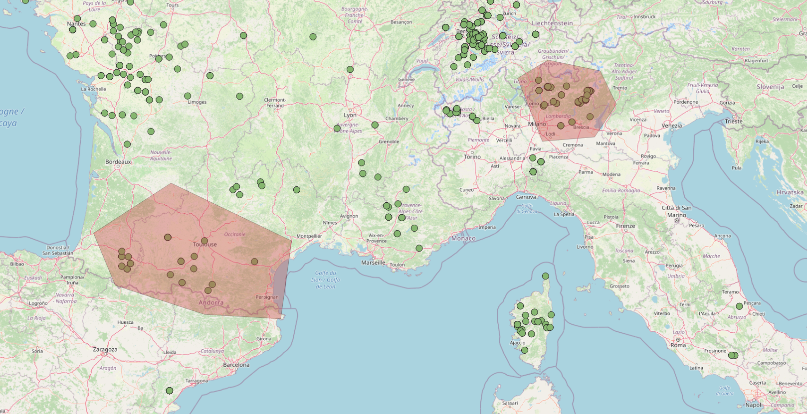
An alternative approach in selecting samples exploits spatial queries. In this example, we imported the goat dataset as geojson file into qgis. Then we created two polygons features in correspondance of the samples we want to collect using GPS coordinates like in the following picture:

select by polygons

Then we exported the two polygons as a shapefile. Here is how we can do a spatial query with st_intersects() in order to collect samples in correspondance of the two areas of interest:

polygons_file <- system.file("extdata", "polygons.shp", package = "smarterapi")
polygons <- sf::st_read(polygons_file)
goat_data <- get_smarter_geojson("Goat", query = list(type = "background"))
sel_sgbp <- sf::st_intersects(goat_data, polygons)
sel_logical <- lengths(sel_sgbp) > 0
selected_goats <- goat_data[sel_logical, ]

The same query could be done using the get_smarter_geojson() function and providing the polygons as an argument:

selected_goats <- get_smarter_geojson(
  "Goat",
  query = list(type = "background"),
  polygons = polygons
)

This means that you can also provide any sf object as a polygon argument. Here we select by country, but using spatial queries:

italy <- rnaturalearth::ne_countries(scale = "medium", returnclass = "sf") %>%
  dplyr::filter(name == "Italy")
italy_goats <- get_smarter_geojson(
  "Goat",
  query = list(type = "background"),
  polygons = italy
)

Convert from MULTIPOINTS to POINT

The get_smarter_geojson() methods returns a sf MULTIPOINTS objects since multiple locations could be collected for each animal, for example for transhumant samples. However, for simplicity, we can focus our analyses using only one GPS coordinate, transforming this MULTIPOINTS object into a POINT object:

hapmap_data <- hapmap_data %>% sf::st_cast("POINT", do_split = FALSE)
hapmap_data
#> Simple feature collection with 92 features and 11 fields
#> Geometry type: POINT
#> Dimension:     XY
#> Bounding box:  xmin: 9.016667 ymin: 37 xmax: 18.16667 ymax: 40.81667
#> Geodetic CRS:  WGS 84
#> # A tibble: 92 × 12
#>    breed      breed_code chip_name    country dataset metadata original_id   sex
#>    <chr>      <chr>      <chr>        <chr>   <chr>   <chr>    <chr>       <int>
#>  1 Altamurana ALT        IlluminaOvi… Italy   "{ \"$… "{ \"lo… ALT1           NA
#>  2 Altamurana ALT        IlluminaOvi… Italy   "{ \"$… "{ \"lo… ALT23          NA
#>  3 Altamurana ALT        IlluminaOvi… Italy   "{ \"$… "{ \"lo… ALT10          NA
#>  4 Altamurana ALT        IlluminaOvi… Italy   "{ \"$… "{ \"lo… ALT20          NA
#>  5 Altamurana ALT        IlluminaOvi… Italy   "{ \"$… "{ \"lo… ALT21          NA
#>  6 Altamurana ALT        IlluminaOvi… Italy   "{ \"$… "{ \"lo… ALT22          NA
#>  7 Altamurana ALT        IlluminaOvi… Italy   "{ \"$… "{ \"lo… ALT15          NA
#>  8 Altamurana ALT        IlluminaOvi… Italy   "{ \"$… "{ \"lo… ALT8           NA
#>  9 Altamurana ALT        IlluminaOvi… Italy   "{ \"$… "{ \"lo… ALT16          NA
#> 10 Altamurana ALT        IlluminaOvi… Italy   "{ \"$… "{ \"lo… ALT24          NA
#> # ℹ 82 more rows
#> # ℹ 4 more variables: smarter_id <chr>, species <chr>, type <chr>,
#> #   geometry <POINT [°]>

The warnings you see in your terminal tell you that you are considering only the first coordinate object from each MULTIPOINT collection.

Visualize SMARTER GPS data

Displaying data using ggplot2

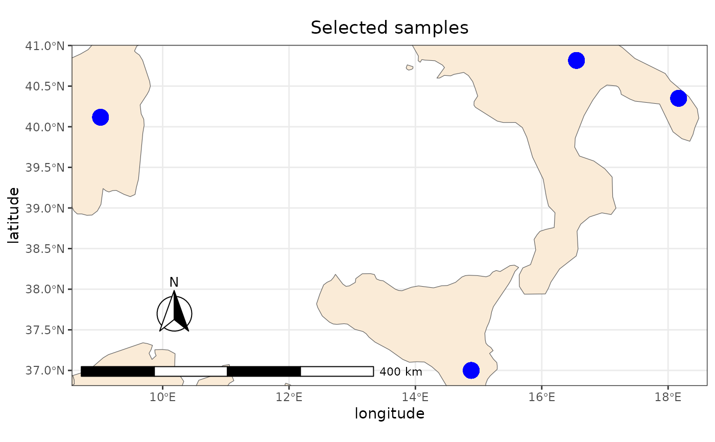
sf data could be visualized using ggplot2. In the following examples we derive the countries from the rnaturalearth package, then we will zoom the plot to the selected points of the previous example:

# determine a bounding box around our samples
bbox <- sf::st_bbox(hapmap_data)

# collect the world countries as sf
world <- rnaturalearth::ne_countries(scale = "medium", returnclass = "sf")

# plot the data: use the bounding box to zoom the plot on our samples
ggplot2::ggplot() +
  ggplot2::geom_sf(data = world, fill = "antiquewhite") +
  ggplot2::geom_sf(data = hapmap_data, color = "blue", size = 5) +
  ggspatial::annotation_scale(location = "bl", width_hint = 0.5) +
  ggspatial::annotation_north_arrow(
    location = "bl",
    which_north = "true",
    pad_x = ggplot2::unit(0.75, "in"),
    pad_y = ggplot2::unit(0.5, "in"),
    style = ggspatial::north_arrow_fancy_orienteering
  ) +
  ggspatial::coord_sf(
    xlim = c(bbox$xmin, bbox$xmax),
    ylim = c(bbox$ymin, bbox$ymax)
  ) +
  ggplot2::theme_bw() +
  ggplot2::theme(plot.title = ggplot2::element_text(hjust = 0.5)) +
  ggplot2::xlab("longitude") + ggplot2::ylab("latitude") +
  ggplot2::ggtitle("Selected samples")

See this post for a nice introduction to sf and ggplot2.

Displaying data using leaflet

Data could be visualized in an interactive way using R leaflet library:

leaflet::leaflet(
  data = hapmap_data,
  options = leaflet::leafletOptions(minZoom = 5, maxZoom = 10)
) %>%
  leaflet::addTiles() %>%
  leaflet::addMarkers(
    clusterOptions = leaflet::markerClusterOptions(), label = ~smarter_id
  )

See Leaflet for R documentation for more information.

Integrate data with external sources

Derive elevation data using elevatr

We can collect elevation data using the elevatr package. The following functions returns the input dataframe with elevation and elev_units as additional columns:

prj_dd <- "EPSG:4326"
hapmap_data_elev <- elevatr::get_elev_point(
  hapmap_data,
  prj = prj_dd,
  src = "aws"
)

See elevatr vignette or elevatr tutorial in rspatialdata documentation for more information and examples.

Add worldclim data from rasters

We can collect data from worldclim database using the geodata package: this package in particular collect raster data from different sources (see geodata reference manual for more information). In this example, we collect the raster with the lowest definition (10min =~ 340km) for worldclim bioclimatic variables and elevation. Raster images will be placed in the tempdir path. Then using terra::extract we calculate the values for our data, after converting them into terra SpatialVectors:

worldclim_bio <- geodata::worldclim_global(
  var = "bio",
  res = 10,
  path = tempdir()
)
bio_data <- terra::extract(worldclim_bio, terra::vect(hapmap_data))

worldclim_elev <- geodata::worldclim_global(
  var = "elev",
  res = 10,
  path = tempdir()
)
elev_data <- terra::extract(worldclim_elev, terra::vect(hapmap_data))

hapmap_data_worldclim <- cbind(hapmap_data, merge(elev_data, bio_data))

See raster extraction from geocomputation with R for more information.